Infrared image non-uniformity correction
NUC (Non-Uniformity Correction) is a key step in the infrared focal plane array (FPA) imaging link to suppress fixed pattern noise (FPN) and improve radiation consistency and subjective perception.
1. Introduction: The necessity of infrared imaging and NUC
Infrared cameras (whether cooled or uncooled) usually use focal plane array (FPA) detectors: each pixel converts incident radiation into an electrical signal, which is read out by circuitry and digitized to form an image. Ideally, the output of all pixels should be exactly the same under the same irradiation; however, in practice, due to factors such as manufacturing process differences, readout link bias, dark current, and temperature drift, different pixels will exhibit different "gains" and "biases," resulting in fixed pattern noise (FPN) such as stripes and patches.
The goal of NUC (non-uniformity correction) is to unify the output of each pixel to the same response scale, remove as much as possible the differences that are independent of the scene and fixed with the pixel, and at the same time try not to lose the details of the real scene and not introduce smear or flicker. For temperature measurement (radiation calibration) systems, stable and traceable NUC is also the basis for temperature inversion accuracy.
Distinguish concepts
NUC mainly deals with "differences between pixels" (spatial fixed terms); adjacent to it are temporal noise suppression (denoising), nonlinear correction, bad pixel repair, radiation calibration (DN → radiation/temperature) and other links. In engineering, they are often combined into a stable imaging pipeline.
2. Sources and manifestations of non-uniformity
2.1 Inconsistent response of detector pixels (gain/offset)
Under the same incident radiation, the conversion efficiency of different pixels is different (gain difference), and the output at zero input is also different (bias difference). The visualization results include: overall graininess, horizontal/vertical stripes, repeated textures with column/row structure, etc.
2.2 Dark current, fixed pattern noise (FPN) and dead pixels
There is a repeatable, fixed component of dark current and readout noise that is superimposed on the image. Dead pixels (dead/hot/noisy) appear as obvious bright spots/dark spots, flickering spots or abnormal noise spots. If not processed, they will interfere with NUC estimation and subsequent enhancement.
2.3 Effects of temperature drift, optical vignetting and readout link
Uncooled detectors and readout circuits are sensitive to temperature, and the gain/offset will drift slowly with chip temperature (or internal temperature); in addition, the optical system may have vignetting, stray light, and lens tube thermal radiation, resulting in global or low-frequency non-uniformity. The readout chain (column amplifiers, ADC channels) also introduces "per-column/per-channel" structured errors.
3. NUC problem modeling
3.1 Linear model (gain-offset)
The most commonly used in engineering is the pixel-level linear response model: represented by the "true radiation response" x on an ideal unified scale, the pixel observation y can be written as:
y = g · x + o + n (g: gain, o: offset, n: time noise)
The core of NUC is to map the original output to the unified domain given the estimated g and o:
x̂ = (y − o) / g (or equivalently scaled to fit a fixed-point implementation)
Here g and o are the respective coefficients of each pixel, which are often saved in a two-dimensional coefficient map (gain map / offset map).
3.2 Nonlinear and high dynamic range models
When the detector/readout becomes nonlinear in high irradiation or high temperature difference scenarios, a simple two-point linear fit will result in residual streaks or temperature measurement deviations. Common practices include:
Piecewise linear: Divide several segments according to DN or temperature range, each segment has two independent points (or linear) parameters, and continuity constraints are applied between segments.
Polynomial/look-up table: Use a higher-order model or LUT to fit the pixel response curve, but control overfitting and noise amplification.
Dual gain/multi-range: When the hardware has multiple gain levels, each level has independent coefficients and handles the consistency of gear switching.
3.3 Time-varying parameters and temperature-related models
For non-refrigeration systems, the "temperature binning/temperature regression" method is commonly used to model:
g = g(T), o = o(T)
where T can be the detector base temperature, internal temperature, or readout plate temperature. In the project, the coefficient maps of multiple temperature points are calibrated offline. During operation, the coefficients are interpolated according to the current temperature or the nearest file is selected, and are supplemented by slow online updates to offset aging and drift.
4. NUC based on calibration plate/black body (offline/online)
Blackbody/uniform radiation sources provide an input that is "as spatially uniform as possible and the radiation is known" and is the classic way to obtain reliable pixel coefficients. According to the number of temperature points provided, common processes are divided into one-point, two-point and multi-point calibration.
4.1 One point correction (offset correction)
When the system gain is stable and the main problem is bias drift (such as overall FPN caused by temperature drift), a single uniform field can be used to obtain the bias map:
Collect multiple frames under a uniform field and perform time domain averaging to obtain the uniform field output y₁ of each pixel.
Use spatial statistics (such as global mean/median or low-pass fit) to obtain the "reference response" r₁.
Set o = y₁ − r₁, and at runtime do x̂ = y − o (or the weighted form).
Advantages:Simple implementation, small coefficient storage; Disadvantages: Unable to correct pixel gain differences, residual stripes are more obvious in scenes with large temperature differences.
4.2 Two-point correction (gain + offset)
The two-point method is the most commonly used NUC calibration method in the industry: use two uniform fields with different temperatures (or radiation intensities) to obtain the output y₁, y₂ of each pixel, corresponding to the reference values r₁, r₂. Then the pixel gain and offset can be estimated as:
g = (y₂ − y₁) / (r₂ − r₁)o = y₁ − g · r₁
When running, press x̂ = (y − o) / g to get the unified scale. If the system needs to perform temperature inversion later, r₁ and r₂ can select "radiation amount corresponding to the blackbody temperature/equivalent DN", and then use the radiation calibration model to complete the mapping of DN → temperature.
4.3 Multi-point correction and piecewise linear/polynomial fitting
Multi-point correction is used to suppress nonlinearity and expand the effective dynamic range. Common engineering strategies:
Segmented two-point method: Covers multiple temperature points, uses two adjacent point parameters in the interval, and selects the interval and interpolates according to the current DN or temperature during runtime.
Pixel-level curve fitting: Fit polynomials or LUTs to each pixel, but strict noise suppression and regularization are required (such as limiting high-order terms, forcing monotonicity).
Reference channel method: Use global reference (mean/median/filtered low frequency) to reduce dependence on absolute radiation accuracy and improve robustness.
4.4 Temperature binning calibration and interpolation strategy
Temperature drift is one of the main reasons for NUC failure. The practical approach is to repeat two-point (or multi-point) calibration at multiple sets of detector temperatures Tₖ to obtain coefficient maps g(Tₖ), o(Tₖ). Runtime:
Nearest Neighbor: Select the closest temperature range, which is fast to calculate but may jump.
Linear interpolation: Interpolates coefficient maps between adjacent temperature bins, smooth but requires more bandwidth.
Separate low frequency and high frequency: high frequency (pixel difference) uses the gear coefficient, and low frequency (vignetting/drift) uses online slow update, thereby reducing the number of temperature gears required.
5. Shutter-Based NUC
The shutter (or baffle) creates an approximately uniform "internal reference field" in front of the lens (usually radiation near the camera's internal temperature) that periodically triggers and updates the bias (and sometimes the gain) while the device is running. This method is very common in uncooled IR because it quickly suppresses FPN that drifts over time.
5.1 Shutter calibration process and parameter update
The typical process is as follows:
Trigger the shutter to close, collect several frames of shutter images and average the time domain y_s.
Construct a reference r_s (e.g. global median, or robust estimate after removing low frequencies).
Update bias: o ← (1−α)·o + α·(y_s − g·r_s) (or equivalent).
Open the shutter and resume imaging.
Among them, α is the update rate, which is usually a smaller value to suppress noise and avoid jumps. If the system only updates the offset, the gain still comes from the offline calibration.
5.2 Shutter frequency, cost and artifact control
Frequency trade-off: The more frequent the shutter, the smaller the drift, but the picture will be blocked (or freeze frames will appear) affecting the experience.
Trigger strategy: It can be triggered by time, temperature change rate, or RNU estimate; the frequency is increased when the temperature changes rapidly.
Artifact control: When there is a large difference between shutter temperature and scene radiation, if the algorithm mistakes the scene structure for non-uniformity, afterimages may be introduced; robust statistics (median/truncated mean) and low-frequency constraints can be used to reduce the risk.
6. Overview of scenario-based NUC (SBNUC) methods
Scene-Based NUC (SBNUC) does not rely on the shutter or external blackbody, but takes advantage of the difference in "moving scenes and relatively fixed non-uniformity" in video sequences to estimate pixel offset/gain through time accumulation and constraints. The advantage is that it does not interrupt the imaging, but the difficulty is to avoid absorbing the real scene texture into the coefficients (causing smear/detail loss).
6.1 Time domain statistics and adaptive filtering
Many SBNUCs treat non-uniformity as a slow variable term and scene changes as a fast variable term, and estimate the bias through low-pass/recursive averaging:
o_t = (1−β)·o_{t−1} + β·(y_t − r_t) (r_t: estimate of the "scene reference" of the current frame)
r_t can be obtained by global statistics, low frequency after local smoothing, or cross-frame fusion after motion compensation. In order to avoid writing edge details into o_t, the update rate is often reduced or a robust loss is used for high gradient areas.
6.2 Motion assistance/registration constraint method
If there is camera shake/translation (or active scanning), the observations of the same scene point on different pixels can be connected through image registration to form a system of equations to estimate the pixel gain and offset. Typical ideas are:
Estimating inter-frame motion (optical flow/feature matching/block matching).
Map multiple frames to the same reference coordinates and establish the constraint that "the same point should be consistent".
Obtain pixel parameters and (optional) scene reflection/radiation maps via least squares or regularized optimization.
This type of method works better when there is sufficient movement and rich texture; it is prone to degradation in static or low-texture scenes.
6.3 Gradient/high-pass constraints and stripe suppression
Streaks often appear as structured low-frequency errors along the row/column direction. In engineering, NUC is often combined with "stripe suppression/de-banding": applying smoothing constraints to the estimated offset map, detrending the column/row structure, or suppressing fixed-direction frequency bands in the frequency domain. However, excessive smoothing should be avoided, which may cause the real low-frequency radiation (vignetting, real temperature gradient) to be weakened.
6.4 Blind correction and regularization optimization framework
A more general blind correction can be written as joint optimization:
min_{x,g,o} Σ‖y − g·x − o‖ + λ·R(x) + μ·S(g,o)
Among them, R(x) constrains the scene (such as total variation TV, sparse gradient), and S(g,o) constrains the smoothness/physical rationality of the coefficient map (such as column consistency, slow change). This framework can unify many SBNUC methods, but online real-time implementation requires a trade-off between accuracy and computational complexity.
7. Dynamic non-uniformity noise correction
This article defines a type of noise that has an obvious stripe structure but is not fixed in the sensor coordinate system and jumps with the frame as dynamic non-uniformity noise (DNU). It is different from traditional FPN/non-uniformity (fixed position, amplitude slowly changes with temperature drift): the spatial form of DNU is usually a bright and dark band in the entire row/column, but its affected row/column index changes with time, making it difficult to completely suppress it with a static NUC coefficient map.
7.1 Cause analysis (why the position jumps)
DNU's "whole row/column jitter" is more commonly caused by non-ideal behavior of system-level links or timing. Typical causes include:
Occasional misalignment of line/frame synchronization analysis: Unstable recognition of line boundary markers such as HSYNC/VSYNC, SOL/EOL, etc., causing some frames to start unpacking or splicing from the wrong starting point of the line, and the structure in the picture jumps with the entire line.
Row-level misalignment caused by data link errors/packet losses: For example, MIPI CSI-2/LVDS may experience packet loss, ECC/CRC errors and recovery when the edge bandwidth or signal integrity is insufficient, manifested as inter-frame jitter in the alignment of the entire row (or row block).
Multi-channel readout (multi-tap) deinterleaving/splicing is unstable: odd and even row and column interleaving, tap boundary splicing, or channel mapping are switched/jittered during operation, causing the strip structure position to jump.
Reference pixel (blind) black level servo/baseline correction instability: If the baseline estimate per frame/row is affected by abnormal references, occlusions, or saturation, visible bias will be introduced in some rows/columns, and the affected index may vary from frame to frame.
DMA/stride/cache switching problem: The row step configuration is inconsistent with the actual pixel stream, and the buffer starting address is accidentally offset at the frame switch, which will produce hopping artifacts for the entire row/column.
7.2 Correction effects and advantages
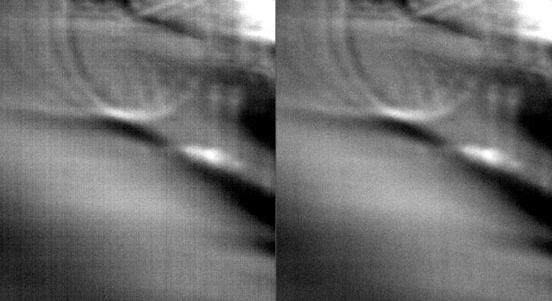
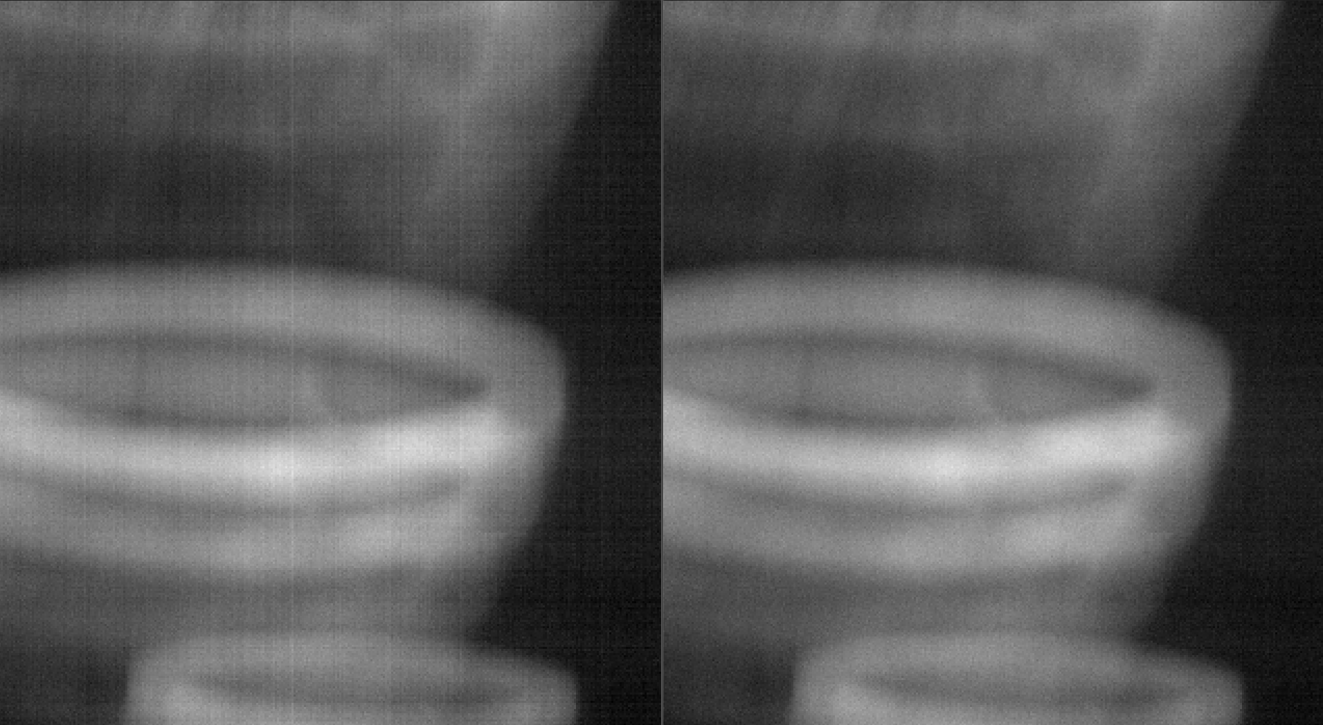
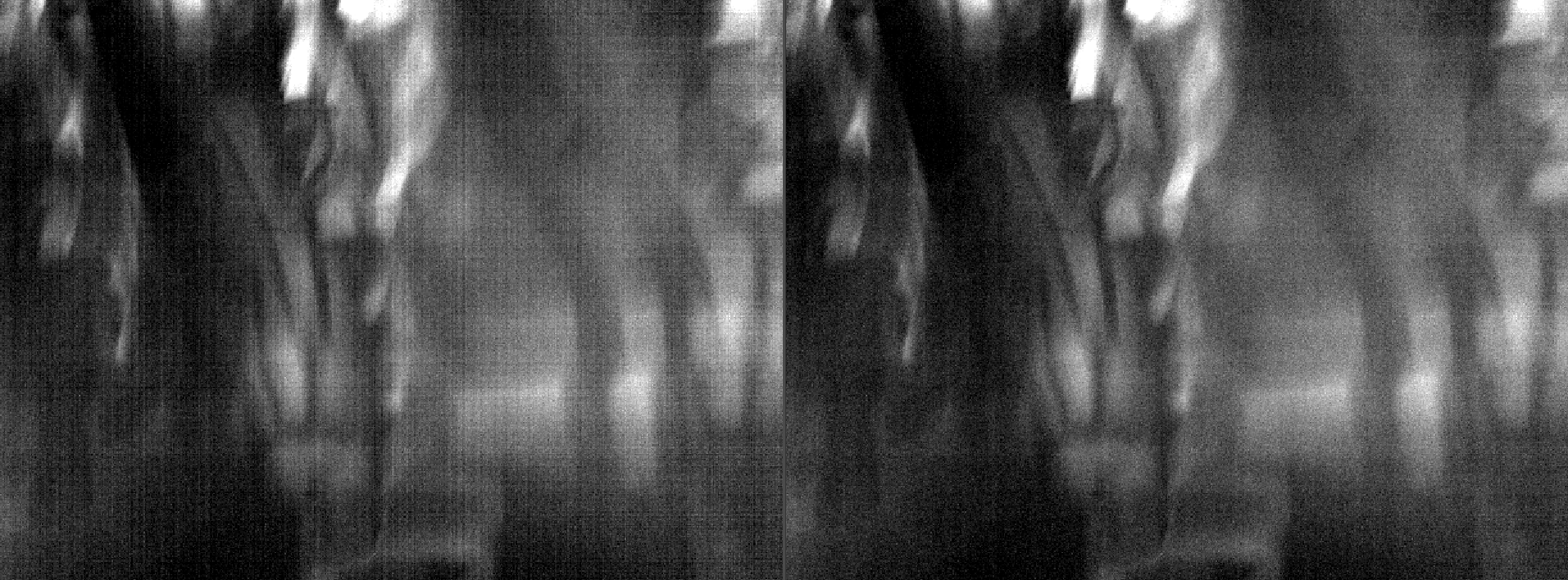
This chapter describes our independently developed dynamic non-uniformity correction algorithm, which performs directional optimization for common problems such as row/column stripes, non-uniformity jumps, and link timing jitter in infrared imaging equipment, emphasizing single-frame robustness and engineering feasibility.
Calibration-free: dynamic stripes can be suppressed by relying entirely on the image's own statistics, without the need for additional blackbody or shutter calibration.
No smear in a single frame: It does not rely on multi-frame accumulation or temporal filtering, and no smear or residual marks are introduced after correction.
Detail-friendly: It suppresses non-uniform noise while maintaining scene details and texture without weakening the real target.
Scene Adaptation: Adapts to scene changes and texture differences, and can stably suppress frame-to-frame changes in stripe positions.
Examples of algorithm effects:
Relationship with NUC
It is recommended to use this DNU correction as "a stripe suppression after NUC": first use offline/shutter NUC to suppress the fixed FPN, and then use this strategy to suppress the row/column stripes with positional jumps, thus covering both static and dynamic non-uniformity artifacts.
8. Dead pixel detection and replacement (collaboration with NUC)
8.1 Types of dead pixels and detection indicators
Bad pixels generally include: always bright/normally dark (response saturation or failure), abnormal noise (excessive variance), flickering points (time instability), and abnormal gain points. The detection can be completed in the offline calibration phase, or incremental detection can be performed during operation. Commonly used indicators:
Uniform field deviation: Sub-threshold difference from neighborhood/global reference under blackbody uniform field.
Time domain variance: multi-frame statistical variance/power spectrum to identify abnormal noise pixels.
Abnormal response curve: The fitting residual at multiple temperature points is too large or the slope is abnormal.
8.2 Spatial interpolation, guided filtering and time domain restoration
Dead pixel replacement is often performed after NUC (to reduce the impact of non-uniformity on the threshold). Methods include:
Neighborhood interpolation: bilinear/bicubic/weighted median, simple and effective for single bad pixels.
Edge preservation: Interpolate in the gradient direction, or use guided filtering/bilateral weights to reduce edge blur.
Temporal fusion: Replace flickering points with robust statistics across multiple frames, but preventing motion-induced ghosting.
9. Summary
The essence of NUC is to make a trade-off between "suppressing fixed pattern noise" and "preserving real radiation/details": offline blackbody calibration provides a high-precision benchmark, shutter correction solves drift during operation, and SBNUC further improves long-term stability without interrupting imaging, but requires stronger robust constraints and engineering protection. Actual systems usually use a combination of "offline two points (or more points) + temperature binning + shutter bias update + bad pixel repair", and continuously monitor quality through a unified indicator system.
This article focuses on proposing and demonstrating our independently developed dynamic non-uniformity correction scheme, which is targeted at common problems such as row/column stripes, non-uniformity jumps, and link timing jitter in infrared imaging equipment. It achieves robust suppression and detail fidelity in a single frame without relying on additional calibration. It can be used as a key reinforcement after NUC to improve overall imaging stability and look and feel consistency.