1. Introduction
1.1 Digital image noise problem
In digital imaging systems, noise is a physical phenomenon that cannot be completely avoided. Whether it's a professional camera or a smartphone, image sensors introduce various noises during the process of converting light signals into electrical signals. These noises appear as random graininess, color spots, or unnatural textures in images, seriously affecting image quality and visual experience.
The impact of noise is particularly obvious in the following scenarios:
- low light environment: Insufficient number of photons leads to reduced signal-to-noise ratio
- High ISO settings: While amplifying the signal, it also amplifies the noise.
- long exposure: Dark current noise accumulation
- Small size sensor: High pixel density and limited photon capture capability of a single pixel
1.2 Why Bayer domain noise reduction is needed
Most digital cameras and smartphones use a Bayer Color Filter Array (CFA) to capture color images. The original image (Raw image) output by the sensor is a single-channel mosaic pattern, and each pixel only records one color information among red (R), green (G) or blue (B).
In the traditional image processing pipeline (ISP Pipeline), noise reduction is usually performed in the RGB domain after demosaicing. However, this approach has obvious flaws:
- Noise propagation: The demosaicing process will use surrounding pixel interpolation, and noise will be propagated and amplified.
- false color: Noise can cause color interpolation errors, producing unnatural color spots
- loss of detail: Noise and real texture are mixed together, and it is difficult to distinguish in the RGB domain
Therefore, direct denoising in the Bayer domain, that is, processing the original image before demosaicing, has become an important research direction in modern ISP.
1.3 Overview of the structure of this article
This article will systematically introduce Bayer noise reduction technology, from basic concepts to advanced algorithms, from theoretical analysis to practical applications. We will discuss the structural characteristics of the Bayer array, the physical sources of noise, the principles and advantages and disadvantages of various noise reduction algorithms, as well as the application of this technology in modern imaging systems, and demonstrate the effect of our BNR algorithm.
2. Basics of Bayer Color Filter Array (CFA)
2.1 Origin and principle of Bayer array
The Bayer color filter array was invented by Kodak scientist Bryce Bayer in 1976 and is currently the most widely used color image sensor solution. The core idea is to take advantage of the human eye's greater sensitivity to green and capture color information by covering the sensor with a specific arrangement of color filters.
- Each pixel is covered by only one color filter (R, G or B)
- Restore complete RGB information through post-algorithmic interpolation
- 50% green pixels, 25% each red and blue
The advantages of this design are:
- Low hardware cost, requiring only a single layer of sensors
- Make full use of human visual characteristics
- Higher spatial resolution
2.2 Arrangement structure of Bayer mode
Standard Bayer arrays use 2×2 repeating units, and common arrangements include RGGB, BGGR, GRBG, and GBRG.
RGGB mode(most common), each 2×2 block contains:
- 1 red pixel (R)
- 2 green pixels (G)
- 1 blue pixel (B)
There are twice as many green pixels as red and blue because the human eye is most sensitive to green (550nm wavelength) and the green channel carries most of the brightness information.
2.3 Characteristics of Raw images
Bayer Raw images have the following characteristics:
- single channel data: Although it contains color information, each pixel has only one intensity value
- mosaic pattern: A checkerboard pattern of alternating red, green and blue colors
- high dynamic range: Usually 10-14 bit linear data, not 8 bit sRGB
- Unprocessed status: Retains the original information of the sensor without white balance, color correction, etc.
- Larger in size: Contains complete sensor information, file size is usually larger
2.4 Differences from RGB full-color images
| Features | Bayer Raw Images | RGB image |
|---|---|---|
| Number of channels | 1 (mosaic) | 3 (R, G, B) |
| information per pixel | 1 color | 3 colors |
| bit depth | 10-14 bit (linear) | 8 bit (after gamma correction) |
| color space | Sensor native | sRGB, Adobe RGB, etc. |
| File format | .raw, .dng, .cr2, etc. | .jpg, .png, .tiff etc. |
| Processing status | raw data | Processed by ISP |
| Editorial flexibility | High (reprocessable) | Low (information is compressed) |
3. Noise characteristics in Bayer images
3.1 Sources of noise
Noise in digital image sensors mainly comes from the following physical processes:
3.1.1 Photon Shot Noise
Cause:The quantum properties of light lead to randomness in the arrival of photons.
Photon shot noise follows a Poisson distribution with a standard deviation equal to the square root of the number of photons. This means that the noise has the following characteristics:
- signal dependence: There is more noise in bright areas and less noise in dark areas.
- It cannot be completely eliminated, it is a basic physical limit
- A major source of noise in sufficient lighting
3.1.2 Read Noise
Cause:Electronic noise during analog-to-digital conversion and circuit readout.
Characteristics of read noise:
- Signal independent: Has nothing to do with light intensity, it is a fixed value
- Main sources: amplifier noise, quantization error, circuit thermal noise
- Dominate in dark areas
- Typical value: 1-10 electrons
Factors affecting read noise include:
- sensor temperature
- Reading speed (frame rate)
- Gain settings (ISO)
- Circuit design quality
3.1.3 Dark Current Noise
Cause:Even in the absence of light, thermal excitation of silicon crystals produces electrons.
Characteristics of dark current noise:
- temperature dependence: For every 6-8°C increase in temperature, dark current doubles
- time dependence: Proportional to exposure time
- Significant in long exposure and high temperature environments
- Typical manifestation: "hot pixels" in long exposure photos
3.1.4 Other noise sources
- Fixed pattern noise (FPN): Uneven pixel response, can be removed by calibration
- Quantization noise: Digitization error of ADC
- 1/f noise: Low-frequency noise, inversely proportional to frequency
- Power supply noise: Interference introduced by the power supply system
3.2 The particularity of Bayer domain noise
The noise of Bayer images has unique spatial structure characteristics:
- Green channel: Larger number of pixels, more reliable noise estimation
- Red and blue channels: sparse pixels, larger noise variance
2. Spatial correlation:
- Pixels of the same color are spatially discontinuous (arranged at intervals)
- Adjacent pixels belong to different channels and have different noise statistical properties.
- Traditional spatial filtering requires special processing
3. Mosaic pattern noise:
- High frequency noise can produce false colors after demosaicing
- Noise near edges can easily be misjudged as texture
- Need to consider the periodicity of the CFA model
3.3 Noise differences in different color channels
Due to physical properties and CFA design, noise behaves differently for each color channel:
| channel | Pixel ratio | quantum efficiency | signal-to-noise ratio | Features |
|---|---|---|---|---|
| Green(G) | 50% | highest | best | Carrying main brightness information, the noise is relatively low |
| Red(R) | 25% | medium | medium | Long wavelength, large penetration depth |
| Blue(B) | 25% | lower | worst | Short wavelength, easily absorbed by surfaces, usually noisiest |
σ²(blue) > σ²(red) > σ²(green1) ≈ σ²(green2)
This difference requires the noise reduction algorithm to adopt adaptive strategies for different channels.
4. Necessity and advantages of Bayer domain noise reduction
4.1 The importance of noise reduction before demosaicing
Demosaicing is a key step in the ISP process, which uses an interpolation algorithm to reconstruct a full-color RGB image from single-channel Bayer data. However, this process is extremely sensitive to noise.
How noise affects demosaicing:
- Interpolation error amplification: Demosaic uses pixels in the surrounding 3×3 or 5×5 area for interpolation, and noise will be propagated to adjacent pixels by the interpolation algorithm. A noise point may affect 9-25 surrounding pixels.
- Edge detection failed: Modern demosaicing algorithms rely on edge detection to select the interpolation direction, and noise can lead to incorrect edge judgments, producing zipper effects and artifacts.
- false color generation: Noise causes color interpolation errors, colored spots appear in gray areas, and colored stripes appear on edges.
- All three RGB channels at this location will be affected
- The surrounding 8 pixels will also be contaminated
- Color deviations of ±15 units may occur
4.2 Avoid noise propagation and artifacts
Noise reduction before demosaicing is equivalent to controlling the source of noise propagation. The benefits of doing this include:
- Prevent false colors: Eliminate noise before it spreads to color channels
- protect edge: Demosaic algorithm can correctly detect edges
- Reduce post-production workload: RGB domain can use milder noise reduction
4.3 Protect edges and details
The key advantage of Bayer domain denoising is the ability to better distinguish between noise and real details.
- Noise pattern is purer: Without interpolation processing, the noise maintains its original statistical characteristics, without interpolation artifacts, and is more in line with the expected noise model (Gaussian, Poisson, etc.).
- Structural information is clearer: The green channel forms a natural brightness map, edges are easier to detect in single-channel data, and the difference in frequency characteristics of texture and noise is more obvious.
- Spatial and frequency domain analysis is more accurate: The periodicity of the CFA pattern can be exploited, the spectral characteristics of the noise are better predicted, and the local statistical estimation is more reliable.
Actual effect:
- Small textures (such as cloth, leaves) are better preserved
- Sharp edges produce no ringing effect
- Low contrast details are not smoothed out
4.4 Comparison with RGB domain noise reduction
| Contrast Dimensions | Bayer domain noise reduction | RGB domain noise reduction |
|---|---|---|
| Processing time | Before mosaic removal | After demosaicing |
| Data volume | Single channel (small) | Three channels (3 times larger) |
| computational complexity | lower | higher |
| noise model | Simple and accurate | Complex, affected by interpolation |
| False color problem | Effectively avoid | difficult to completely eliminate |
| edge protection | Excellent | good |
| Details preserved | Excellent | good |
| color fidelity | high | medium |
| Applicable scenarios | High noise, low light | medium low noise |
• RGB domain noise reduction only: PSNR = 28.5 dB, pseudo-color apparent
• Bayer domain noise reduction only: PSNR = 30.2 dB, better details
• Joint noise reduction: PSNR = 31.8 dB, best visual quality
5. Common Bayer noise reduction algorithms
5.1 Traditional methods
5.1.1 Bilateral Filter
Basic principles:Bilateral filtering combines the similarity in the spatial domain and the value domain to perform a weighted average, taking into account both the spatial distance and the difference in pixel values.
The algorithm uses two Gaussian kernels:
- spatial Gaussian kernel: Calculate the weight based on the spatial distance between pixels
- Range Gaussian Kernel: Calculate weight based on similarity of pixel values
Bayer domain adaptation:
- channel separation: Process R, G, and B channels respectively.
- interval sampling: Pixels of the same color are discontinuous and require skip sampling.
- Adaptive parameters: Adjust the filtering strength according to the noise variance of each channel
- Strong edge protection
- Relatively simple to implement
- Parameters are intuitive and easy to adjust
- High computational complexity
- Easy to over-smooth textured areas
- Parameter selection depends on experience
5.1.2 Non-Local Means (NLM)
Basic principles:Using the self-similarity of the image, similar image patches (patches) are searched within the entire image for weighted averaging.
The core idea of the NLM algorithm is that there are often many similar structures and textures in images. By finding other blocks similar to the current block throughout the image and performing a weighted average of them, the noise can be effectively reduced while retaining details.
Bayer domain improvements:
- CFA-aware block matching: Block matching only compares pixels of the same color, using 4×4 or 6×6 Bayer blocks (full CFA mode included).
- Green channel guidance: First find similar blocks in the green channel (high signal-to-noise ratio), and apply the matching results to the red and blue channels.
- multi-scale strategy: Coarse-scale global search for similar structures, fine-scale local refinement processing.
- Excellent texture retention
- Suitable for processing repeating patterns
- Good denoising effect
- Huge amount of calculation (full image search)
- Poor real-time performance
- May fail in areas of pure noise
Acceleration tips:PatchMatch algorithm (approximate nearest neighbor search), integral graph accelerated block matching, GPU parallel computing, limited search range.
5.1.3 Adaptive noise reduction
Core idea:Adaptively adjust the noise reduction intensity based on local image characteristics (flat areas, edges, textures).
Regional classification strategy:
- flat area(Small local variance): Use strong noise reduction
- edge area(Large gradient): Use weak noise reduction, only along the edge direction
- texture area: Use medium strength noise reduction
- Both details and smooth areas can be considered
- Avoid excessive noise reduction
- Natural visual effect
- Regional classification may be inaccurate
- There are many parameters and the debugging is complicated.
- High reliance on noise estimates
5.2 Frequency domain method
5.2.1 Wavelet transform noise reduction
Basic principles:The wavelet transform decomposes the signal into coefficients of different scales and frequencies. The noise is mainly concentrated in small coefficients at high frequencies, and the real signal is in large coefficients.
Processing flow:
- Wavelet decomposition: Decompose the Bayer image into multiple subbands (LL, LH, HL, HH)
- Coefficient thresholding: Apply a threshold to high-frequency coefficients to remove noise
- Inverse wavelet transform:Reconstruct the denoised image
Threshold method:
- hard threshold: Coefficients smaller than the threshold are set to zero, and coefficients larger than the threshold remain unchanged.
- soft threshold: Set zero if it is less than the threshold, subtract the threshold if it is greater than the threshold
Bayer domain adaptation:
- Channel separation wavelet transform: performed on R, G, and B respectively
- CFA pattern awareness: using special wavelet bases
- Cross-channel coefficient correlation: exploiting the correlation of RGB channels
- Strong multi-scale analysis capabilities
- Solid theoretical foundation
- Suitable for processing textures
- Ringing may occur at the edges
- Limited directional selectivity
- Sensitive to discontinuities in CFA patterns
5.2.2 Frequency domain filtering
Basic principles:Perform low-pass filtering in the frequency domain to suppress high-frequency noise components.
Processing flow:
- Fourier transform the image
- Apply frequency domain filter (low pass filtering)
- Perform the inverse Fourier transform
Common filter types:
- ideal low pass filter: Passes within the cutoff frequency, completely blocks outside the cutoff frequency (may cause ringing)
- Gaussian low pass filter: Smooth transition, better effect (recommended)
- Butterworth filter: between the two
Bayer domain special treatment:
- Bayer mode has specific periodic peaks in the frequency domain
- Need to avoid filtering out structural information of CFA
- Use a notch filter to preserve low and CFA frequencies and suppress pure noise frequencies
- High computational efficiency (FFT is O(N log N))
- Global processing, good consistency
- Easy to understand and implement
- Blurred edges (Gibbs phenomenon)
- Poor airspace selectivity
- Frequency domain features need to be processed for CFA
5.3 Learning-based methods
5.3.1 Deep learning noise reduction network
In recent years, deep learning has made breakthrough progress in the field of Bayer denoising, with performance far exceeding that of traditional methods.
Typical network architecture:
1. DnCNN(Denoising CNN)
Learn from residual noise instead of clean images, use batch normalization to speed up convergence, and employ deep networks (20+ layers). Input a noisy image, output the predicted noise, and the final result is the input minus the predicted noise.
2. U-Net
Adopts an encoder-decoder structure, including multi-scale feature fusion and skip connections. The encoder extracts abstract features through downsampling, the decoder reconstructs details through upsampling, and skip connections retain detailed information.
3. RDN(Residual Dense Network)
Using Dense Block, each layer is connected to all previous layers, making full use of hierarchical features and improving performance through local and global feature fusion.
Bayer domain specific design:
- CFA perceptual convolution: Different color channels use different convolution kernels
- Pixel rearrangement: Rearrange the Bayer mosaic into a 4-channel image (R, G1, G2, B) so that the pixels of each channel are consecutive
- Channel attention mechanism: Adaptively adjust the weight of each color channel
Training strategy:
- Dataset: Synthetic data (clean image + noise model), real data (paired high and low ISO photos), data augmentation (flip, rotate, crop)
- loss function: Combining multiple goals such as pixel loss, perceptual loss, and adversarial loss
- Noise modeling: Simulate the noise characteristics of real cameras (Poisson + Gaussian)
- Best performance (2-5 dB improvement in PSNR)
- Automatically learn features without manual design
- Can be trained end-to-end
- Strong generalization ability (with sufficient training)
- Requires a lot of training data
- Computationally intensive (GPU required for inference)
- The model file is large (tens of MB)
- Poor interpretability
5.3.2 Transformer architecture
Application of Transformer in image noise reduction:
1. Swin Transformer
Using the window attention mechanism, it has a global receptive field, can capture long-range dependencies, is suitable for processing textures and repeated patterns, and the computational complexity is relatively controllable.
2. Restormer
A multi-scale encoding-decoding structure is adopted, combined with multi-head convolutional attention (MDTA) and gated feed-forward network (GDFN), and a progressive learning strategy is used.
3. Hybrid architecture (CNN + Transformer)
- Efficient local feature extraction using CNN at shallow levels
- The middle layer uses Transformer for global relationship modeling
- Detailed reconstruction using CNN in depth
• Diffusion Models: Progressive denoising process to generate high-quality textures
• Neural Operators: Continuous convolution, resolution independent, strong generalization ability
5.4 Combined demosaicing and noise reduction method
Core idea:Simultaneously optimize the two tasks of noise reduction and demosaicing to avoid error propagation in pipeline processing.
Why is joint optimization needed?
- Denoising and demosaicing interact with each other: denoising may smooth textures, affecting edge detection with demosaicing
- Error propagation: Optimizing each module individually can only achieve the local optimum, and the whole may not be the global optimum.
- Artifact accumulation: Pipeline processing accumulates artifacts at each stage
Deep learning end-to-end solution:
Directly from Bayer Raw input to final RGB output, all steps in between are learnable neural network layers. The network learns denoising and demosaicing simultaneously, and is optimized end-to-end through a comprehensive loss function.
Representative work:
- JDD(Joint Demosaicing and Denoising): Dictionary learning method, sparse representation, iterative optimization
- FlexISP: End-to-end can learn ISP, including noise reduction, demosaicing, color correction, and parameters can be fine-tuned
- PyNET: Pyramid network structure, multi-scale processing, optimized for mobile phones
- Avoid error accumulation
- Best performance
- High color fidelity
- Minimal artifacts
- The highest computational complexity
- Training is difficult
- Need pairing data
- Limited model generality (may be sensor-specific)
6. The relationship between noise reduction and demosaicing
6.1 Traditional ISP process
A typical image signal processing (ISP) flow is a multi-stage pipeline:
Noise reduction position selection:
- Bayer domain noise reduction(Raw Denoising):
- Location: Before mosaic removal
- Data: Single Channel Mosaic
- Advantages: Simple noise model, prevents false colors
- Commonly found in: high-end cameras, flagship mobile phone models
- RGB domain noise reduction:
- Location: after demosaic
- Data: Three channels full color
- Advantages: The algorithm is mature and easy to implement
- Commonly found in: mid- to low-end devices
- Multi-stage noise reduction:
- Bayer domain coarse noise reduction → demosaicing → RGB domain fine noise reduction
- Balance performance and efficiency
- Common scenarios for high-end ISPs
6.2 Advantages of joint optimization
Error propagation problem:During separation processing, noise is amplified and propagated through demosaicing interpolation, resulting in false colors that are difficult to completely eliminate in subsequent noise reduction.
Information loss problem:Denoising may over-smooth textures that demosaicing relies on for orientation detection, resulting in edge blurring or zipper artifacts.
Benefits of joint optimization:
| indicator | separation processing | joint optimization | promote |
|---|---|---|---|
| PSNR | 29.5 dB | 31.8 dB | +2.3 dB |
| SSIM | 0.87 | 0.92 | +5.7% |
| false color | obvious | almost none | Significantly |
| edge sharpness | medium | Excellent | obvious |
| processing time | 80 ms | 120 ms | +50% |
6.3 End-to-end processing solution
Definition of end-to-end learning:Directly from Bayer Raw input to final RGB output, all steps in between are learnable neural network layers.
Typical architectural features:
- Bayer feature extraction: Convert mosaic to multi-channel continuous data using pixel rearrangement
- multi-scale coding: Extract features of different scales through downsampling
- adaptive fusion: Attention mechanism learns the weight of each scale
- Upsampling reconstruction: Gradually restore spatial resolution and detail
Training data requirements:
- pairing data: Noisy Raw and clean RGB of the same scene
- Multi-frame average as ground truth
- Different ISO settings (low ISO as GT)
- Compositing: Clean RGB → Analog Raw
- Unpaired data(CycleGAN style): Noisy Raw image set and clean RGB image set, mapped via cycle consistency learning
Actual case:
- Google Pixel: HDR+ pipeline, multi-frame fusion + end-to-end learning
- Apple ProRAW: Retain Raw flexibility + intelligent noise reduction
- Huawei RYYB: Special CFA array + customized neural network
7. Noise reduction effect evaluation
7.1 Objective evaluation indicators
7.1.1 PSNR (peak signal to noise ratio)
Definition:PSNR is the most commonly used objective evaluation index of image quality, which measures image quality by calculating the mean square error (MSE).
PSNR = 10 · log₁₀(MAX²_I / MSE)
MAX_I is the maximum possible pixel value of the image:
• 8-bit image: 255
• 10-bit image: 1023
• Float image [0,1]: 1
Features:
- Unit: dB (decibel)
- Higher is better (generally >30 dB is considered better quality)
- Simple to calculate and widely used
- Does not take into account the visual characteristics of the human eye
- Sensitive to overall brightness shift
- May be inconsistent with subjective feelings
7.1.2 SSIM (structural similarity)
Definition:SSIM compares images from three dimensions: brightness, contrast, and structure, which is more in line with human eye perception.
SSIM takes into account:
- Brightness comparison: Compare the average brightness of two images
- Contrast comparison: Compare the standard deviation of two images
- Structural comparison: Compare the correlation coefficient of two images
- Range: [-1, 1], usually [0, 1]
- Identical when SSIM = 1
- More in line with human eye perception
MS-SSIM (Multi-Scale SSIM):SSIMs are calculated at multiple resolutions and then combined to provide a more comprehensive quality assessment.
7.1.3 Other indicators
LPIPS(Learned Perceptual Image Patch Similarity)
- Similarity based on deep network features
- Closer to human perception
- Use a pre-trained network (such as VGG) to extract features and compare
NIQE(Natural Image Quality Evaluator)
- No reference image quality assessment
- Based on natural image statistics
- No ground truth required
Color fidelity (ΔE)
Calculate color differences in CIE Lab color space:
- ΔE < 1: Hard to detect by human eyes
- ΔE < 3: acceptable
- ΔE > 5: Obvious color difference
7.2 Subjective quality assessment
MOS (Mean Opinion Score) average subjective score
- Invite multiple observers to rate (1-5 points)
- Calculate average score
- 5: Excellent, 4: Good, 3: Average, 2: Poor, 1: Very poor
Pairwise Comparison
- Display two images at the same time
- The observer chooses the better one
- Statistical preference percentage
Assessment Dimensions:
- overall quality: Comprehensive impression
- Noise suppression: Graininess, spots
- Details preserved: Texture, edge definition
- color naturalness: No color cast, false color
- Artifact: Ringing, blocking effect
- Display device calibration (standard sRGB monitor)
- Viewing distance and ambient light control
- Display in random order
- adequate observation time
7.3 Balance between detail preservation and noise suppression
Core contradiction:
- Strong noise reduction → less noise but blurred details
- Weak noise reduction → clear details but residual noise
Evaluation method:
1. Edge Preservation Index (EPI)
Compare edge strength before and after noise reduction:
- EPI ≈ 1: Edge preservation is good
- EPI < 0.8: edges are too smooth
- EPI > 1.2: Possible enhancement artifacts
2. Local analysis of variance
- Texture area: Expected to preserve variance
- Flat region: Desired variance reduction
3. Spectrum analysis
Compare the spectrum before and after noise reduction:
- High Frequency (Detail): Preserved > 70%
- Noise frequency: suppression > 80%
7.4 Color fidelity
Why is color important?
- Noise reduction may change color balance
- Inconsistent processing between channels causes color casts
- False color is a problem specific to Bayer noise reduction
Evaluation method:
1. Grayscale patch color deviation
Select a grayscale area in the test chart, ideally R = G = B, and measure the actual deviation.
2. Color reproduction index (CRI)
Using the Macbeth ColorChecker color chart, the reproduction accuracy of 24 standard color patches was measured.
3. Channel correlation
There is a correlation between the R, G, and B channels of the original image, which should be maintained or slightly improved after noise reduction.
- Average color shift < 2 ΔE
- No obvious false color spots
- Color saturation remains natural
- Inter-channel correlation preserved
8. Practical application scenarios
8.1 Smartphone Photography
Technical challenges:
- Small sensor size:
- 1/2.3" or even smaller
- Single pixel is only 0.8-1.4 μm
- Limited photon capture capability
- Computing resources are limited:
- Needs to run in real time on mobile SoC
- Power consumption limit
- Limited memory bandwidth
- High user expectations:
- Snap and get
- Zero shutter lag
- Image quality comparable to professional cameras
Solution:
1. Multi-frame fusion noise reduction
Continuously shoot 8-16 frames of short-exposure images, perform motion estimation and registration, then weighted average fusion, and finally perform Bayer domain noise reduction.
- Continuous shooting mode: short exposure multiple frames
- Motion estimation and registration
- Robust weighted fusion
- Bayer domain noise reduction
- Final output of high-quality images
2. NPU acceleration
The Neural Processing Unit (NPU) is used to perform Bayer noise reduction and demosaicing, with a processing delay of less than 500ms and no user perception.
3. Adaptive algorithm selection
| scene | Recommended plan | Reason |
|---|---|---|
| Sufficient light | Lightweight bilateral filtering | Fast processing, low power consumption |
| Low light static | Multi-frame fusion | Maximize signal-to-noise ratio |
| Low light dynamics | Single frame deep learning | Avoid motion blur |
Actual case:
- iPhone ProRAW: Retain 12-bit Raw data, apply intelligent noise reduction without destroying dynamic range, and users can fine-tune it later
- Samsung ISOCELL: Pixel binning technology (4-in-1), increasing the amount of light entering a single pixel, combined with AI noise reduction
8.2 Shooting in low light environment
Physical limitations:
- Scene brightness: 1 lux (moonlight level)
- Sensor noise: SNR < 5 dB
- Human eye expectation: SNR > 40 dB
- Needs a 35 dB boost!
Main noise sources:
- Photon shot noise: dominant (fewer photons)
- Read noise: significant (large proportion when signal is weak)
- Dark current: accumulated during long exposures
Technical strategy:
1. Hardware level
- BSI (backside illuminated) sensor: Improve quantum efficiency and reduce light path obstruction
- large pixel size: 1.8 μm or larger, single-pixel photon capture capability improved
- Low read noise design:Double conversion gain (DCG) to reduce analog front-end noise
2. Algorithm level
- Multi-frame long exposure stack: Shoot N frames and align and fuse them, theoretically improving √N times SNR
- Learning night scene enhancement: Single frame extremely low light Bayer Raw input, network learning 100-300 times signal amplification, output bright and clear RGB
- Detect scene brightness and motion
- Adaptively select the number of frames (6-15 frames)
- Automatically set exposure time
- Shoot continuously and align in real time
- weighted fusion
- Bayer domain noise reduction
- Demosaic + Colormapping
- Local tone mapping (HDR)
8.3 High ISO scenes
The essence of ISO:
ISO is a measure of sensor sensitivity. High ISO = amplified sensor signal. ISO 100 to ISO 3200 means the signal is amplified 32x, but the noise is also amplified 32x, and the SNR actually drops.
High ISO noise characteristics:
- color noise: Colored particles, especially in the blue channel
- luminance noise:Grayscale particles
- Fixed pattern noise (FPN): stripes, hot spots
- band noise: Read the periodic noise of the circuit
Noise reduction strategy:
1. ISO immutability design
- Traditional: Front-End Analog Amplification
- Hyundai: Back-end digital amplification
- Advantages: more bit depth is retained, the noise reduction algorithm has more information, and the dynamic range is more flexible
2. Channel separation and noise reduction
Adjust the noise reduction intensity according to the noise variance of each channel. The blue channel is usually the noisiest and requires the most noise reduction.
3. Temporal noise reduction (video)
Using the temporal correlation of consecutive frames, multiple frames are averaged in static areas and smear is avoided in moving areas.
- demand: High-speed shutter (1/1000s+) + high ISO
- challenge: Extremely high noise + need to preserve motion details
- Plan: In-camera hardware-level Bayer noise reduction + post-processing AI noise reduction
- balance:Noise suppression vs. motion clarity
8.4 Medical imaging and scientific imaging
Special requirements:
- Quantitative analysis:
- Pixel values need to accurately reflect physical quantities
- Cannot introduce non-linear distortion
- Small signal differences need to be preserved
- Details matter:
- May be related to diagnostic accuracy
- Small structures (cells, blood vessels) cannot be lost
- High edge sharpness requirements
- Repeatability:
- The same input must produce the same output
- Algorithm parameter determinism
- Traceability
Application areas:
1. Medical X-ray/CT
- Low dose scan → high noise
- Noise reduction reduces patient radiation exposure
- Requirement: Preserve bone/tissue boundaries
- Method: iterative denoising, balancing fidelity term and smoothing regularization term
2. Fluorescence Microscopy
- Low light + high magnification → very low SNR
- Signal level: 50-200 photons/pixel
- Noise: Poisson + read noise
- Requirements: Quantitative measurement of fluorescence intensity
- Solution: Scientific grade CCD (cooled, low noise), statistical modeling noise reduction, 3D noise reduction (using z-stack)
3. Astrophotography
- Very long exposure (several hours)
- Dark current and thermal noise are significant
- Weak signals (distant galaxies)
- Technology: dark field subtraction, flat field correction, multiple stacking, very gentle Bayer noise reduction (preserving real stars)
- FDA/CFDA certification requirements
- Algorithm validation and clinical trials
- Cannot "beautify" the image (may mask lesions)
- Doctor’s final judgment is required
9. Summary
9.1 Key points of Bayer noise reduction
Through the systematic introduction of this article, we can summarize the core points of Bayer noise reduction:
Theoretical basis:
- Bayer arrays are the foundation of modern digital imaging, capturing color information using an RGGB mosaic pattern
- Image noise originates from physical processes such as photon shot noise, read noise, and dark current noise.
- The noise characteristics of different color channels are significantly different and require adaptive processing.
Technical advantages:
- Noise reduction before demosaic can effectively prevent noise propagation and false color generation
- The noise model in the Bayer domain is simpler, more accurate, and easier to model and process.
- Reduce the quality requirements for demosaicing algorithms and improve overall ISP performance
Method evolution:
Practical experience:
- There is no universal noise reduction algorithm, it needs to be selected according to the scene.
- Parameter tuning requires a balance between noise suppression and detail preservation
- Assessment needs to combine objective indicators (PSNR, SSIM) and subjective quality
- Real-time applications need to consider computational complexity and hardware resources
9.2 Suggestions for choosing a noise reduction solution
Scenario-driven choices:
| Application scenarios | Recommended plan | Reason |
|---|---|---|
| Smartphone (daily) | Lightweight CNN + multi-frame fusion | Balance performance and power consumption |
| Smartphone (Night View) | Multi-frame alignment + deep learning | Extreme noise reduction capability |
| professional camera | Adaptive NLM + optional AI | Quality first, user controllable |
| real time video | Fast bilateral + temporal noise reduction | Latency sensitive |
| medical imaging | Conservative noise reduction + edge protection | Accuracy is crucial |
| scientific imaging | Noise reduction based on statistical models | Quantitative analysis needs |
Resource constraints considerations:
- Sufficient computing resources (server/PC): Deep learning method, high quality, can be processed offline
- Mobile devices (cell phones/embedded):Lightweight network + hardware acceleration, or optimized version of traditional methods
- Extremely low power consumption (IoT/wearable devices): Simple filtering, or noise reduction only at key frames
Suggestions during the development phase:
- prototype stage: Use mature libraries (OpenCV, scikit-image) to quickly verify the effect and establish performance benchmarks
- Optimization stage: Optimize for the target platform, consider parallelization (SIMD, GPU), quantization and pruning (deep learning)
- product stage: Fully test various scenarios, user-adjustable parameters (optional), and continuously collect feedback and optimization
9.3 Outlook
Technology development direction:
- Deep Fusion of Computational Photography: No longer pure noise reduction, but overall image enhancement, multi-modal fusion (RGB + depth + event camera), and intelligent processing driven by scene understanding
- Personalization and Adaptation:Learn user preferences, automatically adapt to the shooting environment, and continue online learning
- Hardware and software co-design: Dedicated AI ISP chip, algorithm and hardware joint optimization, breaking through power consumption and performance bottlenecks
- New sensor technology: Quad Bayer/Nonacell (pixel binning), quantum dot sensor (higher quantum efficiency), event-driven sensor (ultra-high dynamic range)
Unsolved challenges:
- Extreme scenes: Ultra low light (< 0.001 lux), ultra high speed (> 1000 fps), ultra high resolution (> 100 MP)
- A balance between authenticity and beautification: AI noise reduction may "illusion" details. How to ensure the authenticity of images? Ethical and Legal Considerations
- Universality and specialization: One model fits all cameras? Or customized for each sensor? Meta-learning may be the answer
Bayer noise reduction technology has undergone tremendous changes from simple filtering to today's deep learning. It is not only a technical issue of image processing, but also a cross-fusion of optics, electronics, computer science and artificial intelligence.
As mobile devices become the main imaging tool and the era of computational photography arrives, the importance of Bayer noise reduction becomes increasingly apparent. In the future, with the advancement of AI technology, the popularization of dedicated hardware, and the emergence of new sensors, we have reason to believe that we can obtain clear, natural, and detailed high-quality images even under extremely harsh shooting conditions.
For engineers and researchers engaged in image processing, computer vision, or photography technology, a deep understanding of the principles and practices of Bayer noise reduction will be a key part of mastering modern imaging systems.
10.BNR algorithm effect display
Our BNR (Bayer Noise Reduction) algorithm is optimized for real shooting scenes. While suppressing high ISO and low-light noise, it focuses on maintaining edge structure and texture details, reducing over-smoothing and false color problems common with traditional methods.
10.1 Algorithm goals and characteristics
- Noise suppression: For signal-related noise modeling in the Bayer domain, adaptively adjust the denoising intensity
- Detail protection: Reduce filtering intensity in edge and texture areas, retaining structural information
- color stable: Suppress the propagation of color noise and reduce the risk of false colors in the subsequent demosaicing stage
- The project can be implemented: Taking into account both image quality and computational complexity, it can be integrated into ISP real-time links
10.2 Visual effect example (before denoising vs after denoising)
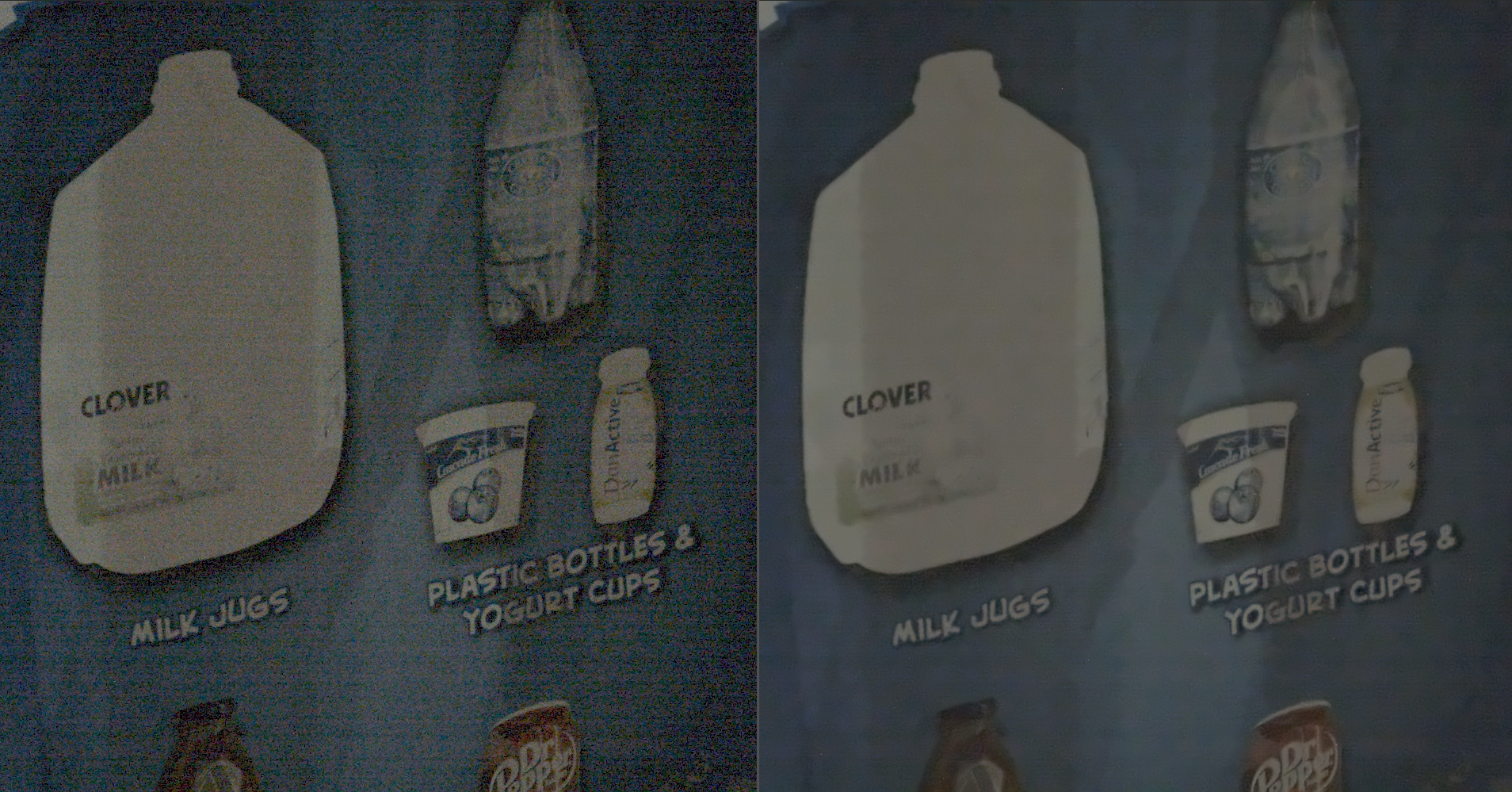
Figure 10-1: Comparison of BNR algorithm effects (left: before denoising, right: after denoising)
From the above comparison, it can be seen that the random grain noise of the denoised image is significantly reduced, while the subject outline and text information maintain good readability, which reflects the algorithm's ability to balance between "noise reduction intensity" and "detail fidelity".